Compile models (i.e. especially equations) once and simulate them afterwards without having to resort to runtime symbolic algebra or numeric differentiation.

Build a semantic analysis upon this foundation. Distinguish between compile-time, link-time and run-time checks.

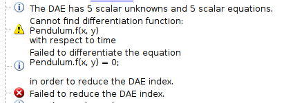
model Pendulum Real x(start=0.1),y(start=0.9, fixed=true),vx,vy,F; equation x^2 + y^2 = 1; vx = der(x); vy = der(y); der(vx) = F*x; der(vy) = F*y - 9.81; end Pendulum;

model Pendulum function f input Real x; input Real y; output Real r; algorithm r := x^2 + y^2 - 1; end f; Real x(start=0.1),y(start=0.9, fixed=true),vx,vy,F; equation f(x,y) = 0; vx = der(x); vy = der(y); der(vx) = F*x; der(vy) = F*y - 9.81; end Pendulum;

model Pendulum function f input Real x; input Real y; output Real r; algorithm if (x <> 0) then r := x^2 + y^2 - 1; else if (y <> 0) then r := y^2 - 1; else r := -1; end if; end if; end f; Real x(start=0.1),y(start=0.9, fixed=true),vx,vy,F; equation f(x,y) = 0; vx = der(x); vy = der(y); der(vx) = F*x; der(vy) = F*y - 9.81; end Pendulum;

Consider the ideal representation of the cartesian Pendulum: $$\begin{align} x^2 + y^2 &=& 1\\ \ddot{x} &=& F x \\ \ddot{y} &=& F y - 9.81 \end{align}$$

The dual Problem (in LP sense) to the assignment problem introduces slack variables $\bar{c}, \bar{d}$ and a consistency condition: $$d_j - c_i \geq \sigma_{ij}$$

where $\sigma_{ij}$ is the highest derivative of variable $j$ in equation $i$

The interpretation of $c_i$ is the "index" of equation $i$, i.e. the number of times it needs to be derived, $d_j$ is the (maximal) degree of derivation of variable $j$ in the model.

The dual goal is to minimize: $$\sum d_j - \sum c_i$$

Incidence matrix: $$\sigma = \begin{vmatrix} {\color{grey} x} & {\color{grey} y} & {\color{grey} F} & \\ 0 & 0 & - \infty & {\color{grey} x^2 + y2 - 1} \\ 2 & -\infty & 0 & {\color{grey} \ddot{x} - Fx} \\ -\infty & 2 & 0 & \color{grey} \ddot{y} - Fy + 9.81\\ \end{vmatrix}$$

Solution: $$\begin{align*} \bar{c} &=& (2,0,0)\\ \bar{d} &=& (2,2,0)\\ \end{align*}$$

Sorting derived equations: $$\begin{align} x &\mapsto& x^2 + y^2 &=& 1\\ \dot{x} &\mapsto& x\dot{x} + y\dot{y} &=& 0\\ \ddot{x} &\mapsto& {\dot{x}}^2 + x \ddot{x} + {\dot{y}}^2 + y \ddot{y} &=& 0\\ F &\mapsto& \ddot{x} &=& F x \\ \ddot{y} &\mapsto& \ddot{y} &=& F y - 9.81 \end{align}$$

Note, that $\ddot{y}, \ddot{x}, F$ form a connected component

We start with a small term language $t$ $$\begin{aligned} \tau ::= & \unk{n}{d} & | & \tau \oplus \tau \\ | & \tau \otimes \tau & | & \phi ~ \tau \\ | & \mathbb{R} \end{aligned}$$

$\tau \in t$, $\phi$ is one of a set of primitive functions, $\unk{n}{d}$ are unknowns, $n, d \in \mathbb{N}$

(obviously not turing-complete)

Let $\mathbb{D} \subseteq \mathbb{R}$ be an open interval, $\bar{x} = (x_1 \ldots x_p) \in \xdomain$ be a vector containing $n$-times differentiable real valued functions on that interval.

Strict evaluation relation: $\env \tau \reduce\ r$ indicates that $\tau$ evaluates to $r$ under $\envonly$, where $v \in\mathbb{D}$ is the independent variable.

$$\frac{}{\env \mathtt{u}_{n,k} \reduce \der{k}{x_n}(v)}{n \leq p}$$

$$\frac{\env \tau_1 \reduce r_1 ~~ \env \tau_2 \reduce r_2}{\env \tau_1 \oplus \tau_2 \reduce (r_1 + r_2)}$$

Let $f : \xdomain \times \mathbb{D} \rightarrow \mathbb{R}$ an $n$-times differentiable function, then: $$\env \tau \leadsto f \Leftrightarrow \env \tau \reduce f(\bar{x}, v)$$

($\tau$ computes $f$)

To include AD, we parameterize $t$ over the order of total differentiation $n$ and number of parameters $p$: $$\begin{aligned} \tau^{(n,p)} ::= & \unk{m}{k} & | & \tau^{(n,p)} \oplus \tau^{(n,p)} \\ | & \tau^{(n,p)} \otimes \tau^{(n,p)} & | & \phi ~ \tau^{(n,p)} \\ | & \mathbb{R}^{n+1 , p+1} \\ \end{aligned}$$

There is a simple relation $\lceil r \rceil^{(n,p)}$ which lifts $t$-terms into $\tnp$-terms.

General Idea: Generalize Automatic Differentiation (e.g. Dual Numbers) to Derivative Matrices $$\Dermatrix{n}{p}{f} = \begin{vmatrix} \partial_{j} \der{i} f(\bar{x}, v) \end{vmatrix} \in \mathbb{R}^{n+1,p+1}$$

Where: $$\begin{align*} \partial_0 f &=& f \\ \partial_j f &=& \frac{\partial f}{\partial x_j}, ~~ i \in 1 \ldots p\\ \der{i} f &=& \frac{\mathtt{d}^i f}{\mathtt{d}v^i} \\ \end{align*}$$

$$\begin{align*} I \begin{vmatrix} r_{0,0} & \cdots & r_{0,p} \\ \vdots & \ddots & \vdots \\ r_{n,0} & \cdots & r_{n,p} \\ \end{vmatrix} &= \begin{vmatrix} r_{0,0} & \cdots & r_{0,p} \\ \vdots & \ddots & \vdots \\ r_{n-1,0} & \cdots & r_{n-1,p} \\ \end{vmatrix} \\ \\ \end{align*}$$

$$\begin{align*} \Delta \begin{vmatrix} r_{0,0} & \cdots & r_{0,p} \\ \vdots & \ddots & \vdots \\ r_{n,0} & \cdots & r_{n,p} \\ \end{vmatrix} &= \begin{vmatrix} r_{1,0} & \cdots & r_{1,p} \\ \vdots & \ddots & \vdots \\ r_{n,0} & \cdots & r_{n,p} \\ \end{vmatrix} \end{align*}$$

Again, a strict big step semantics $\redad{n}$ $$\frac{}{\env \unk{m}{k} \redad{n} \Dermatrix{n}{p}{\der{k} x_m}}$$

AD-Evaluation of a term yields correct total and partial derivatives. $$\env \tau \leadsto f \Rightarrow \env \lift{n}{p}{\tau} \redad{n} \Dermatrixshort{n}{p}{f}$$

Addition is simply matrix-addition $$\frac{\begin{align*}\env \tau_1 \redad{n} A \\ \env \tau_2 \redad{n} B\end{align*}}{\env \tau_1 \oplus \tau_2 \redad{n} A + B}$$

Multiplication is defined recursively $$\frac{\begin{align*}\env \tau_1 \redad{0} \bar{a} \\ \env \tau_2 \redad{0} \bar{b} \end{align*}} {\env \tau_1 \otimes \tau_2 \redad{0} \bar{a} \Multop \bar{b}}$$

$$\begin{align*} (\bar{a} \Multop \bar{b})_0 &= a_0 \times b_0 & \\ (\bar{a} \Multop \bar{b})_i &= a_i \times b_0 + b_i \times a_0 & i \in 1 \ldots p \end{align*}$$

$$\frac{\begin{align*} \env &\tau_1 \redad{n+1} A \\ \env &\tau_2 \redad{n+1} B \\ \env \Delta(A)& \otimes I(B) \redad{n} C \\ \env \Delta(B)& \otimes I(A) \redad{n} D\end{align*}} {\env \tau_1 \otimes \tau_2 \redad{n+1} \begin{vmatrix} A_0 \Multop B_0 \\ C + D \end{vmatrix}}$$

AD allows for precise, arbitrary order derivation of precompiled terms

This means, we can compile any equation into $t^{(n,p)}$ and decide during runtime, what $n$ and $p$ is required.

Questions?